
Malaria Cells Image Classification With Residual Neural Network
This article describes my own attempt to automate the process of diagnosis by building an image classifier based on a residual neural network. Properly trained, it may significantly improve the quality of the diagnosis and automate the process thus freeing the humans for other tasks.
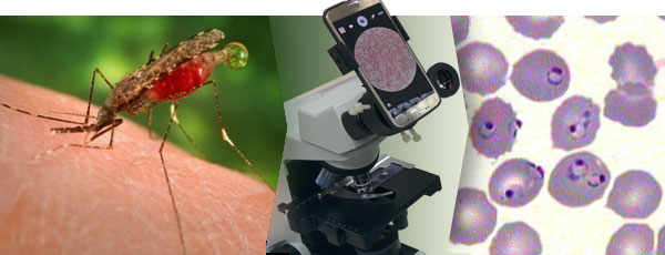
Malaria stays a global health problem — about 200 million cases worldwide, and causing about 400,000 deaths per year. It is caused by parasites that are transmitted through the bites of infected mosquitoes. Most deaths occur among children in Africa, where a child dies from malaria almost every minute. Besides malaria is a leading cause of childhood neuro-disability.
Thanks to existing drugs, malaria nowadays is a curable disease. However inadequate diagnostics and emerging drug resistance are the major barriers to successful deaths reduction.
One of the promising solutions — is the development of a fast and reliable diagnostic test, along with better treatment, development of new malaria vaccines, and mosquito control.
The current standard method for malaria diagnosis in the field is based on blood films analysis using a light microscope. Thus, about 170 million blood films are examined every year for malaria, which involves manual counting of parasites.
Accurate parasite counts are essential to diagnosing malaria correctly, testing for drug-resistance, measuring drug-effectiveness, and classifying disease severity. However, microscopic diagnostics is not standardized and depends heavily on the experience and skill of the microscopist.
Thus incorrect diagnostic decisions in the field are not rare. For false negative cases, this means unnecessary use of antibiotics, a second consultation, lost days of work, and in some cases progression into severe malaria. For false positive cases, a misdiagnosis entails unnecessary use of anti-malaria drugs and suffering from their potential side-effects, such as nausea, abdominal pain, diarrhea, and sometimes severe complications.
This project
My project is inspired by the work of the Communications Engineering Branch (CEB) of the Lister Hill National Center for Biomedical Communications, an R&D division of the U.S. National Library of Medicine.
This article describes my own attempt to automate the process of diagnosis by building an image classifier based on a residual neural network. Properly trained, it may significantly improve the quality of the diagnosis and automate the process thus freeing the humans for other tasks.
Dataset
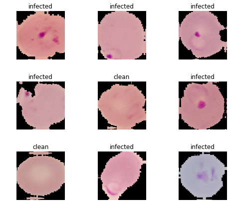
The dataset provided is balanced — consists of a total of 27,558 cell images with equal instances of parasitized (infected) and uninfected (clean) cells. For the model training/validation the data set was split in 80/20 ratio.
Training:   22047 items
Validation:  5511 items
Model 1 — ResNet-34
ResNet-34. Stage 1 – Training the last layer only
We will grab a pre-trained model and train it’s last layer on our data. We will use accuracy as metric.
learn = create_cnn(data, models.resnet34, pretrained=True,    metrics=accuracy)
learn.fit_one_cycle(8)
Total time: 17:28
+-------+------------+------------+----------+
| epoch | train_loss | valid_loss | accuracy |
+-------+------------+------------+----------+
|     1 |   0.252428 |   0.177682 | 0.937761 |
|     2 |   0.179210 |   0.141670 | 0.952459 |
|     3 |   0.154940 |   0.112976 | 0.958810 |
|     4 |   0.132179 |   0.110817 | 0.958265 |
|     5 |   0.131507 |   0.100075 | 0.962620 |
|     6 |   0.111973 |   0.096983 | 0.964435 |
|     7 |   0.109729 |   0.095398 | 0.963890 |
|     8 |   0.117686 |   0.095875 | 0.964979 |
+-------+------------+------------+----------+
The best accuracy at Stage 1 = 0.964979. And some of the most incorrectly classified images:
ResNet-34. Stage 2 – Unfreezing all layers, fine-tuning, and choosing learning rate
Now we will “unfreeze” all the layers, select the learning rate and train the whole model again.
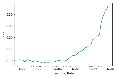
To ensure most effective training, we choose a proper learning rate — approximately one degree less than at the point of increase.
The learning rate we will use at this point will range from 1e-6 to 1e-5.
learn.unfreeze()
learn.fit_one_cycle(4, max_lr=slice(1e-6,1e-5))
Total time: 11:54
+-------+------------+------------+----------+
| epoch | train_loss | valid_loss | accuracy |
+-------+------------+------------+----------+
|     1 |   0.112082 |   0.093375 | 0.966068 |
|     2 |   0.113694 |   0.091406 | 0.966612 |
|     3 |   0.111754 |   0.089694 | 0.967157 |
|     4 |   0.103694 |   0.089652 | 0.966975 |
+-------+------------+------------+----------+
The final accuracy achieved at this point = 0.966975. It is not the best, though: the accuracy at epoch 3 was better. Nevertheless, the accuracy of the ResNet-34 model at Stage 2 has slightly increased.
Here is how the confusion matrix looks like:
ResNet-34. Stage 2. Confusion matrix.

This means:
- 101 out of 2764 (3.65 %) infected cells were classified as clean — False Negative;
- 81 out of 2747 (2.95 %) clean cells were classified as infected — False Positive.
And some of the most incorrectly classified images:
Model 2 — ResNet-50
Now we will grab another model with more — 50 layers — ResNet-50, also pre-trained.
ResNet-50 Stage 1. Training the last layer only
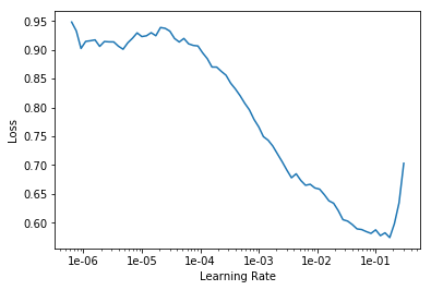
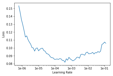
To ensure most effective training, we choose a proper learning rate — approximately one degree less than at the point of increase:
Then we training the model for eight epochs with the learning rate selected:
learn.fit_one_cycle(8, max_lr=1e-2)
Total time: 37:32
+-------+------------+------------+----------+
| epoch | train_loss | valid_loss | accuracy |
+-------+------------+------------+----------+
|     1 |   0.185371 |   0.147972 | 0.951370 |
|     2 |   0.171672 |   0.137128 | 0.958084 |
|     3 |   0.144841 |   0.118323 | 0.958084 |
|     4 |   0.145557 |   0.136532 | 0.950281 |
|     5 |   0.120406 |   0.104959 | 0.964072 |
|     6 |   0.113034 |   0.096068 | 0.967338 |
|     7 |   0.093753 |   0.093459 | 0.968064 |
|     8 |   0.078344 |   0.091585 | 0.967882 |
+-------+------------+------------+----------+
The final result achieved with ResNet-50 at Stage 1 — accuracy = 0.967882. It is not the best, though.
ResNet-50. Stage 2 – Unfreezing, fine-tuning, and learning rates
For Stage 2 we will now unfreeze all layers of the ResNet-50 model and train it again with the manually selected learning rate.
learn.unfreeze()
learn.fit_one_cycle(4, max_lr=slice(2e-5,1e-4))
Total time: 24:43
+-------+------------+------------+----------+
| epoch | train_loss | valid_loss | accuracy |
+-------+------------+------------+----------+
|     1 |   0.102057 |   0.098065 | 0.966249 |
|     2 |   0.112881 |   0.095750 | 0.965342 |
|     3 |   0.095904 |   0.092911 | 0.967701 |
|     4 |   0.067358 |   0.089976 | 0.966975 |
+-------+------------+------------+----------+
The best result achieved with ResNet-50 at Stage 2 — accuracy = 0.966975.
Here is how the confusion matrix looks like:
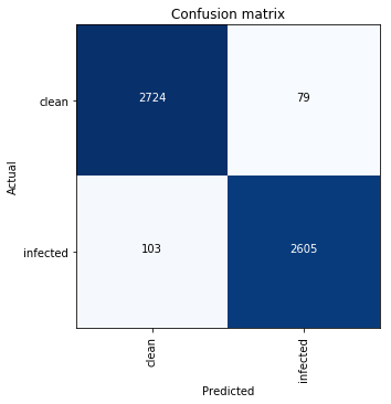
This means:
- 103 out of 2708 (3.8 %) infected cells were classified as clean — False Negative;
- 79 out of 2803 (2.82 %) clean cells were classified as infected — False Positive.
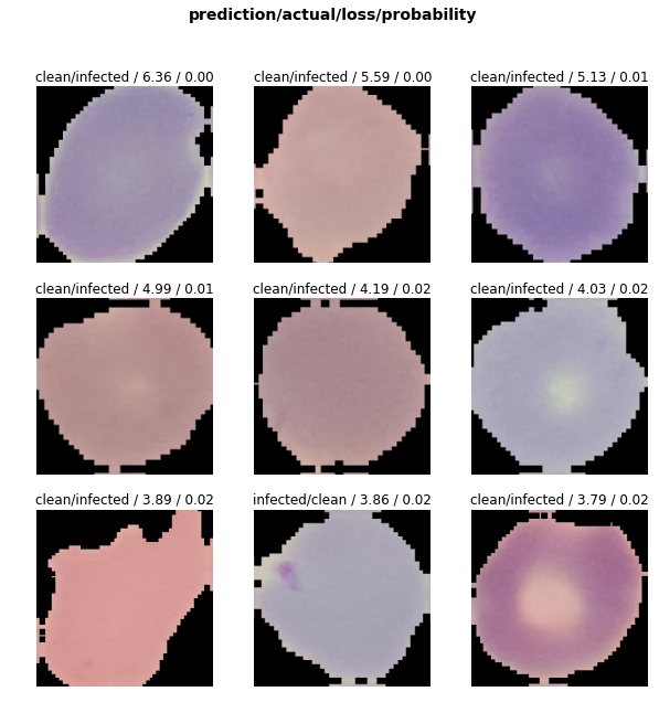
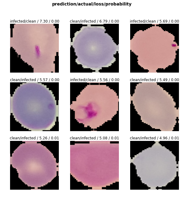
And some of the most incorrectly classified images:
Conclusions
- Looking at the ResNet-50. Stage 2. Incorrectly classified images, we may conclude that some of the images in fact may be incorrectly labeled in the dataset — those which are clearly infected are labeled as clean and vice versa.
- Training accuracy achieved with both models is comparable:
+-----------+---------+----------+
|   Model   |  Stage  | Accuracy |
+-----------+---------+----------+
| ResNet-34 | Stage 1 | 0.964979 |
| ResNet-34 | Stage 2 | 0.966975 |
| --------- | ------- | -------- |
| ResNet-50 | Stage 1 | 0.967882 |
| ResNet-50 | Stage 2 | 0.966975 |
+-----------+---------+----------+
However, the ResNet-50 at Stage 1 is more accurate. Thus we can load the model saved at the Stage 1 and use as is or continue to train it again with different hyper-parameters like another learning rate to achieve yet better results.
- Training time per epoch depends both on the model complexity — number of layers, and on the number of layers trained (one last layer at Stage 1 vs. all layers at Stage 2). Besides, it may correlate with the batch size — smaller batch size (32 vs. 64) was used for the ResNet-50.
+-----------+---------+-----------------------------+
|   Model   |  Stage  | Average time per epoch, sec |
+-----------+---------+-----------------------------+
| ResNet-34 | Stage 1 |           131.0             |
| ResNet-34 | Stage 2 |           178.5             |
| --------- | ------- | --------------------------- |
| ResNet-50 | Stage 1 |           281.5             |
| ResNet-50 | Stage 2 |           370.75            |
+-----------+---------+-----------------------------+
Tools used
The fast.ai library (v. 1.0.38) build on top of the PyTorch was used. The model was trained on a virtual machine running on the Google Cloud Platform.
Machine type: n1-standard-4 (4 vCPUs, 15 GB memory) GPU: 1 x NVIDIA Tesla K80
Sources
The Jupyter notebook is available in repository on GitHub.